Discount Rate

In the Present Value sessions, we “discounted” the future cash flow to today’s value by 3%.

Because it’s the rate to discount the cash flow, it is called a Discount Rate. So, the formula I wrote in the present value session can be rewritten like this:

☟

But, for that exercise, why did we use 3% as the discount rate?

Let’s recall what I wrote in the Assumption session: in finance, you are assuming that “whenever you have cash, you deposit it in a bank to enjoy compound interest”. And in the present value session, we used an interest rate of 3%. So, whenever you received cash, you deposited in your bank where you “expected” cash balance to increase by 3% compound interest. By the same token, when you paid out cash, you forwent a chance of enjoying such compound interest effect (because your account had lesser cash balance due to the pay out) because you “expected” that you are going to earn something in return. And because the process of deriving a present value was to remove (=discount) such compound interest effect based on your expectation, we used 3% as the discount rate.

From this, we can say this:

“The discount rate you use to discount future cash flow depends on how much you expect to earn from your cash receipts and how much you expect to earn in return from your cash payments by forgoing a chance to earn compound interest”

In the previous case, for example, your bank offered an interest of 3%. So, if you are receiving cash, you could “expect” your cash to grow compoundly by 3%. But when you are paying out cash, you forwent a chance to enjoy such 3% compound interest for the decision you made, “expecting” what you are paying for will at least worth that much. Hence, this 3% was your expectation. And, because you are either receiving cash with or paying cash with such expectations, those expectations are considered in finance a “cost”. (you see, when you pay $5 for a banana, you expect it to taste good. So that you are paying $5 for your expectation and, hence, it’s a cost.) 

Now. Don’t you think it’d be so easy if you could know for certain how much you could expect to earn from your cash and how much return you could expect from payments? Absolutely. But, unfortunately, that’s not the case in business. Why? Because of many reasons, which, in most cases, are uncertain. For example, interest rate could fluctuates; it can go up or can go down along the way. You also need to account for expectations of other investors, not only yours, which also changes over time or based on their financial condition. You might even need to take into consideration returns of other investment opportunities on the table, each of which also has its uncertainties, and so on. So….besides the expectation, or the “cost”, you also need to add a factor of uncertainties, which we call it “risk”.

Given all that, we can rephrase the above quote like this:

“The discount rate must reflect "cost” and “risk”. 

Sounds finance, doesn’t it? I know there are many people who think “what!?…so we need to quantify all the costs and the risk now!? Ewww…” Well, I have a bad news and a good news for you. The bad news is “yes, you need to”. And the good news is “thanks to those bright minds, there are tools you can use to calculate them.

Cost of Equity: Capital Asset Pricing Model (CAPM)

Let me start off with more complicated one, which is the cost of equity. Like I mentioned before, when it comes to business, cash has expectations attached to it. And in case of equity, “investors’ expectations” are the cost. Why? Because your investors are investing their cash to your business when they should have other opportunities to invest on other business or projects. That means, when the investors decide to invest in yours, they are expecting that they are going to earn certain returns. (if they expect lesser returns from you than other investments, why invest in you, right?)

And a commonly used tool to calculate the cost of equity is a formula called Capital Asset Pricing Model, or CAPM. And it goes like this:

I know……I hate seeing some Greek letters in a formula, too. It does look intimidating. But, don’t worry. To be very honest, you don’t need to calculate for every variables to complete the exercise. What you mainly have to do is…look for them.

But before taking a closer look on the formula itself, let me explain first what it does for you. It helps you derive the cost of equity of a certain business or a company by taking into consideration how it has been performing in relative to some benchmarks.

Try to imagine this (yes, really try to imagine it). You are in a class of 100 students. And there’d been many exams. The teacher always tells the class “if you don’t study at all, you are likely to score 40/100”. Because none of you want to fail, you study. But each student, including yourself, studies for different hours, so the class’s overall score varies by exams. After few years, you gather all the data and noticed there’s a certain “trend” in how you score: for exams where the class’s average score is high, your score tends to be higher than the average, but whenever the class’s average is low, you tend to score even lower. So, your score tends to move along the class average, but the variation is “magnified (when the class gets high scores and you get higher score. the class gets low score and you get even lower scores)”. When you quantify such trend, you found out that your score is always higher than 40/100 by the amount of 1.2 multiplied by the different between the class’s average (where everyone studies for random hours) and the 40/100 (with zero study hours). Now, the teacher announces that there’ll be a final exam next month, and you want to predict how you do at it. You talk with other students and find out that they are going to study as usual and expecting to get an average of 75/100. From the previous analysis, therefore, you can expect your score will be 86 (=40 + 1.3 (75-40)).

So…what happened here is you analyzed your score trend in relative to the class to predict your expected performance for the next exam.

In a nutshell, that’s what the CAPM does. In other words, CAPM can be explained like this:

You analyze the “trend” of the historical return of the company’s securities in relative to the market, so once you know what the overall market’s expected return is, you can figure out how much return the investors are likely to be expecting from you.

You might wonder “why do we pay attention to the return of the company’s securities when I just want to find out the cost of equity…?”. As I mentioned in the earlier part of this session, the cost of equity is the expectation of and risks to the investors. And when the investors participate in your business or invest in your project, they buy your stocks. Hence, the cost of equity can be rephrased as “how much return the investors are expecting and how much risk they will anticipate when they purchase your stocks (securities)”. In short, the CAPM assumes that the stocks are good representation of expectations and risks.

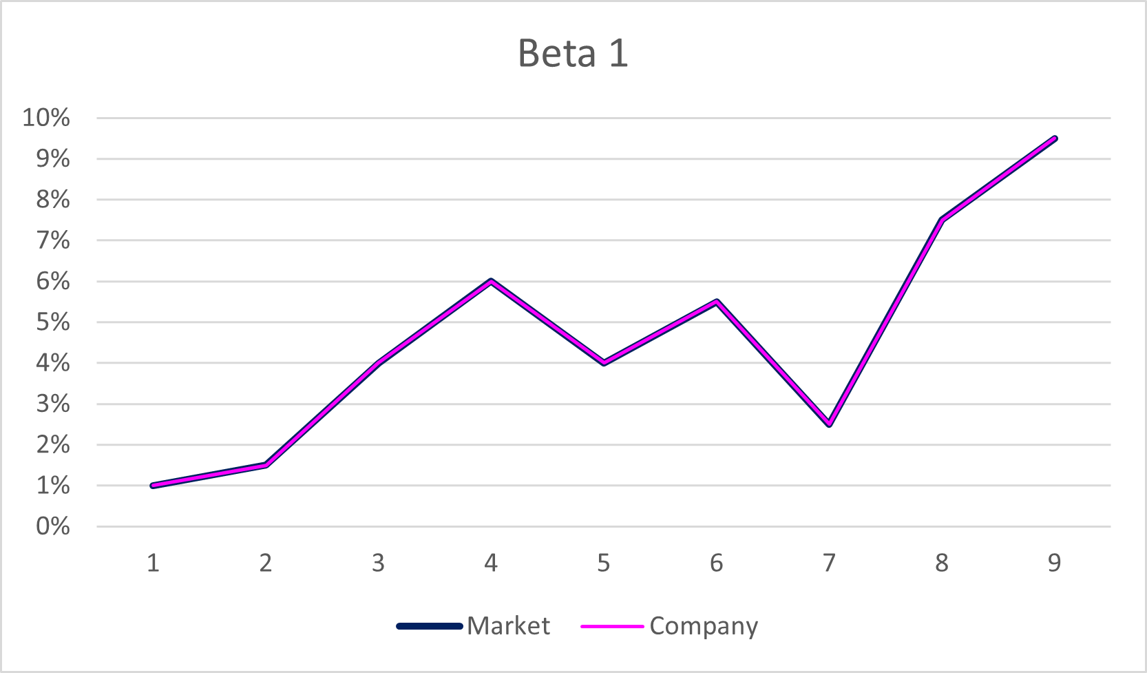
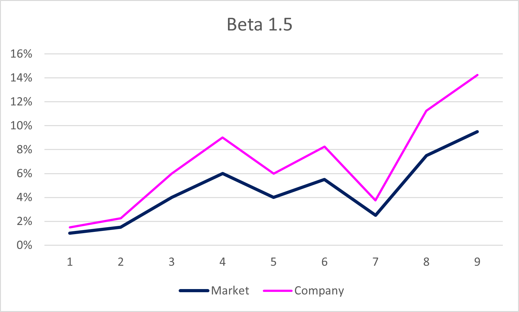
Now, let’s go back to the phrase above in bold. The “trend” of how your company’s securities do in relative to the market is known as “volatility”, and is expressed in a formula as Beta (β). And for Beta, there’s 2 things you should remember: the first one is “1”, and the second one is “plus and minus”. When the beta is “1”, this means the “trend” of the return of your security is the same as the trend of the market. If market goes up, your securities go up by the same degree (ex. market up by 1%, your security up by 1%). When the market goes down, yours go down at the same level. If beta is larger than 1, the trend of your stock is magnified compared to that of the market (ex. market up by 1%, your security up by more than 1%). If lower than 1, the return of your stock fluctuate in lesser manner than the market (ex. market up by 1%, yours up by less than 1%). And when the sign is “+ (plus)”, it means your stock moves in the same direction as the market (ex. market up, yours up), and when the sign is “- (minus)”, your stock moves in the opposite direction as the market (market up, yours down). Combining both, when the beta is “+1”, it means the fluctuation of your stock is the same as that of the market. If, say, the beta is “-1.5”, your stock moves in the opposite direction from the market, with even larger fluctuation (ex. market 1%, your stock down by 1.5%).

Here are some examples:

Yes. There is a way to calculate beta for a company. But, let me refrain from going in there for now. Instead, please note that if you are analyzing a beta for a publicly traded company, you can find beta on the internet. Search “beta company (name)”.

Next, the 40/100 score in the class example is known as “risk-free” because you can get that score even without any study hours (so there’s no risk), which is expressed as “rf”. And, the class’s expected score on the final exam is an analogy for the market’s expected return, or the “E(rm)”. If you can figure out these 3 variables (β, E(rm) and rf), then you can plug them into the formula and derive the expected return for YOUR company’s securities, or the cost of equity.

To relieve your stress, I have some good news: There’s representative numbers out there that are typically used in finance for E(rm) and rf.

For E(rm), in case of US, we typically use “average historical return of S&P 500”. Why? Because S&P 500 is composed of 500, large, stable companies from variety of industries, so is considered well diversified, hence a good benchmark. Of course returns fluctuate every year even for S&P, but that is why we take historical return, assuming it’s a good indicator of the market. For rf, we need to know the return of risk-free (zero risk. safest) security, and the most commonly used indicator is US 10-year Treasury Bond. I know there many comments out there questioning it, but in general, we consider the return of US 10-year Treasury Bond to be the risk-free rate. (I can explain more details for the E(rm) and rf, but to avoid any confusion, I want you to just remember so.)

Like beta, you can Google these variables by, say, “S&P 500 average return” or “US 10 year treasury bond yield”.

With all that in mind, let’s worn on an exercise, though it’ll be relatively easy; search, plug and calculate.

Let’s say you are trying to discount a cash flow for….Coca Cola. Then the beta, according to the online search, is 0.55. Hence the cost of equity will be like this:

Voila! What this means is that the investor for Coca Cola is expecting 7.2% return, hence is the cost of equity. (Needless to say, I’m using Coca Cola just to show you how to calculate the cost of equity. So, please don’t use this to estimate stock value and blame me if you lost the bet…)

Please note that each variables (β, expected market return and risk-free rate) can be derived by more rigorous analysis and/or calculation. But, since the purpose of this website is to explain to you the very basics of finance terms, especially on what each means, allow me to refrain from going super detail on them. Consider this as “a translator of translators”.

Cost of Debt

If you have single debt, then “interest expense / total debt” is the same as the interest rate. But if you had multiple debts, then you need sum interest expenses and divide by the total debt. So the formula can be broken down like this:

As always, let me give you a quick exercise. Say a company pays 3% on $100,000 loan and 5% on $75,000 loan. And the tax rate is 30%. What would the cost of debt for this company be?

When you keep studying for both cost of equity and cost of debt, you might notice that cost of equity is usually higher than cost of debt. Recall earlier that I said earlier “cost of cash reflects risks”. Debt is considered less risky compared to equity because the lender reserves the right to be paid back prior to equities, so is considered safer, hence the cost is lower. On the other hand, the equity is riskier because there’s no assurance of returns and, in case of a default, the equity investor is the last people to be paid back. Therefore, is costlier.

Now. You have studied the ways to calculate cost of equity and cost of debt. Then, what do you do with it?

If you are planning to deploy only an equity or fund a project with only a debt, it’s simple. Just use any cost of equity of cost of debt you derived as the cost of capital. However, in reality is not typical. In most cases, you use combinations of equity and debt. So, in order to know the cost of capital, you need to combine them with weights.

……Huh!?

Welcome to the final topic for this session: weighted average cost of capital.

Weighted Average Cost of Capital (WACC)

As a starter, let me redefine this quite “financy” jargon for you.

WACC is a tool to “incorporate and balance the weight (=Weighted Average) of cost and risk associated (=Cost) with (of) cash (Capital).”

So…

The WACC is a formula that helps you weigh the cost of equity and the cost of debt, combine them and derive a single rate, which the cost of capital.

Let me give you an analogy here so you can depict what WACC does. I’m quite sure many of you have used color paints. Do you remember a situation where you wanted to paint a leaf but didn’t have green on your palette? What did you do? Sure, you mixed blue paint and yellow paint. And to make darker green, you added more blue than yellow, whereas more yellow than blue when you wanted lighter green. Plus, because you are mixing blue (darker color) and yellow (lighter color), the final color will not be either darker than the original blue nor lighter than the original yellow.

This is what WACC does, but not with yellow and blue, but with cost of equity and cost of debt. So, through WACC, you are adding cost of equity and cost of debt, and the final outcome, or the cost of capital, will be somewhere between the cost of equity and the cost of debt (not above riskier cost of equity and not below less risky debt). Hence, if the amount of equity is exactly the same as the amount of debt, the cost of capital will exactly be the average of the two costs. But, if the amount of equity is more than the amount of debt, then the cost of capital will be higher than the average.

With that in mind, let’s take a look at the WACC formula:

At a glance, it looks like another complex formula. But if you pay attention, you can notice that it’s not. First, “Re” is the cost of equity, which you already know how to calculate. And Rd is the cost of debt, which, again, you know how to derive. Second, E is the amount of equity and D is the amount of debt. So, what “E/(E+D)” and “D/(E+D)” are doing is simply calculating how much each source of cash weighs compared to the total. By multiplying the cost of equity and its weight, you can derive how much the cost of equity (or blue from the above sample) is weighed on the final outcome (darkness of green). You do the same for cost of debt, and add them both to get the cost of capital.

Here’s an example. Let’s say you decide to implement a project. You plan to inject $100 equity and $80 debt. The cost of equity is 8%, while the cost of debt is 4% (after accounting for a tax shield). Let’s calculate what the cost of capital would be:

So, IF you injected the same amount of equity and debt, then the cost of capital was 6%, the average of 8% and 4%. However, because you deployed more equity amount than the debt (so, skewed towards the riskier side), the cost of capital is higher than the average.

Congratulations. Now you know how to calculate the cost of capital, or the discount rate. Quite easy, right?